3. SE(3): 3D Transformations

The group of all proper rigid transformations (rototranslations) in 3D Cartesian space is \(SE(3)\) (SE: special Euclidean group). Transformations consist of a rotation and a translation. Those can be represented in different ways just like rotations can be expressed in different ways. The minimum number of components that are required to describe any transformation from \(SE(3)\) is 6.

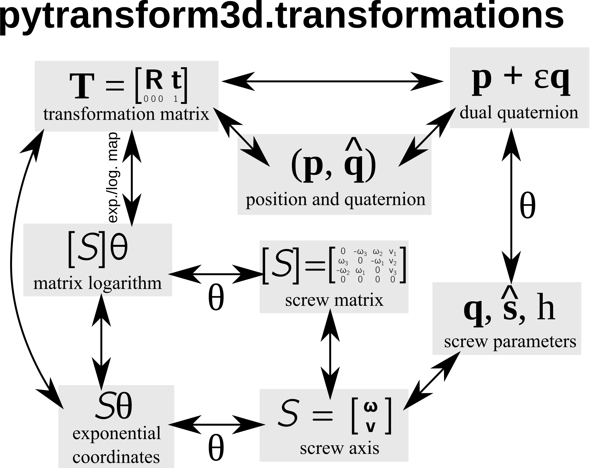
Overview of the representations and the conversions between them that are available in pytransform3d.

For most representations of orientations we can find an analogous representation of transformations:

• A transformation matrix \(\boldsymbol T\) is similar to a rotation matrix \(\boldsymbol R\).

• A screw axis \(\mathcal S\) is similar to a rotation axis \(\hat{\boldsymbol{\omega}}\).

• A screw matrix \(\left[\mathcal{S}\right]\) is similar to a cross-product matrix of a unit rotation axis \(\left[\hat{\boldsymbol{\omega}}\right]\).

• The logarithm of a transformation \(\left[\mathcal{S}\right] \theta\) is similar to a cross-product matrix of the angle-axis representation \(\left[\hat{\boldsymbol{\omega}}\right] \theta\).

• The exponential coordinates \(\mathcal{S} \theta\) for rigid body motions are similar to exponential coordinates \(\hat{\boldsymbol{\omega}} \theta\) for rotations (compact axis-angle representation / rotation vector).

• A twist \(\mathcal V = \mathcal{S} \dot{\theta}\) is similar to angular velocity \(\hat{\boldsymbol{\omega}} \dot{\theta}\).

• A (unit) dual quaternion \(p_w + p_x i + p_y j + p_z k + \epsilon (q_w + q_x i + q_y j + q_z k)\) is similar to a (unit) quaternion \(w + x i + y j + z k\).

Not all representations support all operations directly without conversion to another representation. The following table is an overview.

Representation	Inverse	Transformation of vector	Concatenation	Interpolation	Renormalization
Transformation matrix \(\pmb{R}\)	Inverse	Yes	Yes	No	Required
Exponential coordinates \(\mathcal{S}\theta\)	Negative	No	No	ScLERP	Not necessary
Logarithm of transformation \(\left[\mathcal{S}\theta\right]\)	Negative	No	No	No	Not necessary
Position and quaternion \((\pmb{p}, \pmb{q})\)	No	No	No	No	Required
Dual quaternion \(\boldsymbol{\sigma}\)	Quaternion Conjugate	Yes	Yes	ScLERP	Required

3.1. Transformation Matrix

One of the most convenient ways to represent transformations are transformation matrices. A transformation matrix is a 4x4 matrix of the form

\[\begin{split}\boldsymbol T = \left( \begin{array}{cc} \boldsymbol R & \boldsymbol t\\ \boldsymbol 0 & 1\\ \end{array} \right) = \left( \begin{matrix} r_{11} & r_{12} & r_{13} & t_1\\ r_{21} & r_{22} & r_{23} & t_2\\ r_{31} & r_{32} & r_{33} & t_3\\ 0 & 0 & 0 & 1\\ \end{matrix} \right) \in SE(3).\end{split}\]

It is a partitioned matrix with a 3x3 rotation matrix \(\boldsymbol R\) and a column vector \(\boldsymbol t\) that represents the translation. It is also sometimes called the homogeneous representation of a transformation. All transformation matrices of this form generate the special Euclidean group \(SE(3)\), that is,

\[\begin{split}SE(3) = \{ \boldsymbol{T} = \left( \begin{array}{cc} \boldsymbol{R} & \boldsymbol{t}\\ \boldsymbol{0} & 1 \end{array} \right) \in \mathbb{R}^{4 \times 4} | \boldsymbol{R} \in SO(3), \boldsymbol{t} \in \mathbb{R}^3 \}.\end{split}\]

pytransform3d uses a numpy array of shape (4, 4) to represent transformation matrices and typically we use the variable name A2B for a transformation matrix, where A corrsponds to the frame from which it transforms and B to the frame to which it transforms.

It is possible to transform position vectors or direction vectors with it. Position vectors are represented as a column vector \(\left( x,y,z,1 \right)^T\). This will activate the translation part of the transformation in a matrix multiplication (see vector_to_point()). When we transform a direction vector, we want to deactivate the translation by setting the last component to zero (see vector_to_direction()): \(\left( x,y,z,0 \right)^T\).

We can use a transformation matrix \(\boldsymbol T_{BA}\) to transform a point \({_A}\boldsymbol{p}\) from frame \(A\) to frame \(B\):

\[\begin{split}\boldsymbol{T}_{BA} {_A}\boldsymbol{p} = \left( \begin{array}{c} \boldsymbol{R}_{BA} {_A}\boldsymbol{p} + {_B}\boldsymbol{t}_{BA}\\ 1\\ \end{array} \right) = {_B}\boldsymbol{p}.\end{split}\]

You can use transform() to apply a transformation matrix to a homogeneous vector.

Pros

• Supported operations: all except interpolation.

• Interpretation: each column represents either a basis vector or the translation.

• Singularities: none.

Cons

• Rrepresentation: 16 values for 6 degrees of freedom.

• Renormalization: inherited from rotation matrix.

3.2. Position and Quaternion

An alternative to transformation matrices is the representation in a 7-dimensional vector that consists of the translation and a rotation quaternion:

\[\left( x, y, z, q_w, q_x, q_y, q_z \right)^T\]

This representation is more compact than a transformation matrix and is particularly useful if you want to represent a sequence of poses in a 2D array.

pytransform3d uses a numpy array of shape (7,) to represent position and quaternion and typically we use the variable name pq.

Pros

• Representation: compact.

Cons

• Supported operation: translation and rotation component are separated and have to be handled individually.

3.3. Screw Parameters

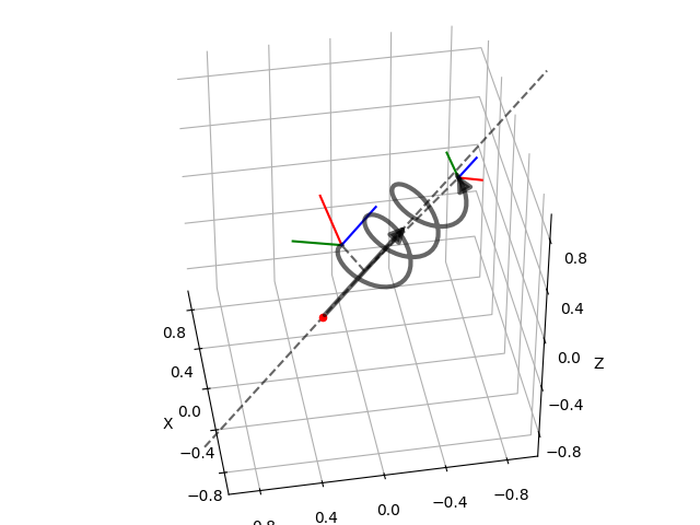
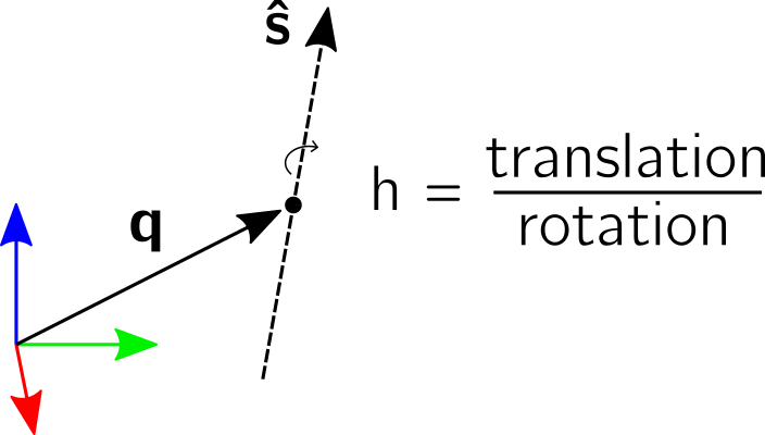
Just like any rotation can be expressed as a rotation by an angle about a 3D unit vector, any transformation (rotation and translation) can be expressed by a motion along a screw axis [2] [3] [4]. The screw parameters that describe a screw axis include a point vector \(\boldsymbol{q}\) through which the screw axis passes, a (unit) direction vector \(\hat{\boldsymbol{s}}\) that indicates the direction of the axis, and the pitch \(h\). The pitch represents the ratio of translation and rotation. A screw motion translates along the screw axis and rotates about it.

pytransform3d uses two vectors q and s_axis of shape (3,) and a scalar h to represent the parameters of a screw.

3.4. Screw Axis

A screw axis is typically represented by \(\mathcal{S} = \left[\begin{array}{c}\boldsymbol{\omega}\\\boldsymbol{v}\end{array}\right] \in \mathbb{R}^6\), where either

1. \(||\boldsymbol{\omega}|| = 1\) or

2. \(||\boldsymbol{\omega}|| = 0\) and \(||\boldsymbol{v}|| = 1\) (only translation).

pytransform3d uses a numpy array of shape (6,) to represent a screw axis and typically we use the variable name S or screw_axis.

In case 1, we can compute the screw axis from screw parameters \((\boldsymbol{q}, \hat{\boldsymbol{s}}, h)\) as

\[\begin{split}\mathcal{S} = \left[ \begin{array}{c}\hat{\boldsymbol{s}} \\ \boldsymbol{q} \times \hat{\boldsymbol{s}} + h \hat{\boldsymbol{s}}\end{array} \right]\end{split}\]

In case 2, \(h\) is infinite and we directly translate along \(\hat{\boldsymbol{s}}\).

3.5. Exponential Coordinates

By multiplication with an additional parameter \(\theta\) we can then define a complete transformation through its exponential coordinates \(\mathcal{S} \theta = \left[\begin{array}{c}\boldsymbol{\omega}\theta\\\boldsymbol{v}\theta\end{array}\right] \in \mathbb{R}^6\). This is a minimal representation as it only needs 6 values.

pytransform3d uses a numpy array of shape (6,) to represent a exponential coordinates of transformation and typically we use the variable name Stheta.

Warning

Note that we use the screw theory definition of exponential coordinates and \(se(3)\) (see next section) used by Lynch and Park (2017) [1], and Corke (2017) [2]. They separate the parameter \(\theta\) from the screw axis. Additionally, they use the first three components to encode rotation and the last three components to encode translation. There is an alternative definition used by Eade (2017) [3] and Sola et al. (2018) [4]. They use a different order of the 3D vector components and they do not separate \(\theta\) from the screw axis in their notation.

Pros

• Representation: minimal.

• Supported operations: interpolation; can also represent spatial velocity and acceleration.

Cons

• Supported operations: concatenation and transformation of vectors requires conversion to another representation.

3.6. Logarithm of Transformation

Alternatively, we can represent a screw axis \(\mathcal S\) in a matrix

\[\begin{split}\left[\mathcal S\right] = \left( \begin{array}{cc} \left[\boldsymbol{\omega}\right] & \boldsymbol v\\ \boldsymbol 0 & 0\\ \end{array} \right) = \left( \begin{matrix} 0 & -\omega_3 & \omega_2 & v_1\\ \omega_3 & 0 & -\omega_1 & v_2\\ -\omega_2 & \omega_1 & 0 & v_3\\ 0 & 0 & 0 & 0\\ \end{matrix} \right) \in se(3) \subset \mathbb{R}^{4 \times 4}\end{split}\]

that contains the cross-product matrix of its orientation part and its translation part. This is the matrix representation of a screw axis and we will also refer to it as screw matrix in the API.

pytransform3d uses a numpy array of shape (4, 4) to represent a screw matrix and typically we use the variable name screw_matrix.

By multiplication with \(\theta\) we can again generate a full description of a transformation \(\left[\mathcal{S}\right] \theta \in se(3)\), which is the matrix logarithm of a transformation matrix and \(se(3)\) is the Lie algebra of Lie group \(SE(3)\).

pytransform3d uses a numpy array of shape (4, 4) to represent the logarithm of a transformation and typically we use the variable name transform_log.

3.7. Twist

We call spatial velocity (translation and rotation) twist. Similarly to the matrix logarithm, a twist \(\mathcal{V} = \mathcal{S} \dot{\theta}\) is described by a screw axis \(\mathcal S\) and a scalar \(\dot{\theta}\) and \(\left[\mathcal{V}\right] = \left[\mathcal{S}\right] \dot{\theta} \in se(3)\) is the matrix representation of a twist.

3.8. Dual Quaternions

Similarly to unit quaternions for rotations, unit dual quaternions are an alternative to represent transformations [5] [6] [7]. They support similar operations as transformation matrices.

A dual quaternion consists of a real quaternion and a dual quaternion:

\[\boldsymbol{\sigma} = \boldsymbol{p} + \epsilon \boldsymbol{q} = p_w + p_x i + p_y j + p_z k + \epsilon (q_w + q_x i + q_y j + q_z k),\]

where \(\epsilon^2 = 0\) and \(\epsilon \neq 0\). We use unit dual quaternions to represent transformations. In this case, the real quaternion is a unit quaternion and the dual quaternion is orthogonal to the real quaternion. The real quaternion is used to represent the rotation and the dual quaternion contains information about the rotation and translation.

Dual quaternions support similar operations as transformation matrices: inversion through the conjugate of the two individual quaternions dq_q_conj(), concatenation through concatenate_dual_quaternions(), and transformation of a point by dq_prod_vector(). They can be renormalized efficiently (with check_dual_quaternion()), and interpolation between two dual quaternions is possible (with dual_quaternion_sclerp()).

Warning

The unit dual quaternions \(\boldsymbol{\sigma} = \boldsymbol{p} + \epsilon \boldsymbol{q}\) and \(-\boldsymbol{\sigma}\) represent exactly the same transformation.

The reason for this ambiguity is that the real quaternion \(\boldsymbol{p}\) represents the orientation component, the dual quaternion encodes the translation component as \(\boldsymbol{q} = 0.5 \boldsymbol{t} \boldsymbol{p}\), where \(\boldsymbol{t}\) is a quaternion with the translation in the vector component and the scalar 0, and rotation quaternions have the same ambiguity.

Pros

• Representation: compact.

• Renormalization: cheap in comparison to transformation matrix.

• Supported operations: all, including interpolation with ScLERP.

• Computational efficiency: the dual quaternion product is slightly cheaper than the matrix product.

• Singularities: none.

Cons

• Interpretation: not straightforward.

• Ambiguities: double cover.

3.9. References

[1]

Lynch, K. M., Park, F. C. (2017). Modern Robotics. http://hades.mech.northwestern.edu/index.php/Modern_Robotics

[2] (1,2)

Corke, P. (2017). Robotics, Vision and Control, 2nd Edition, https://link.springer.com/book/10.1007/978-3-319-54413-7

[3] (1,2)

Eade, E. (2017). Lie Groups for 2D and 3D Transformations. https://ethaneade.com/lie.pdf

[4] (1,2)

Sola, J., Deray, J., Atchuthan, D. (2018). A micro Lie theory for state estimation in robotics. Technical Report. http://www.iri.upc.edu/files/scidoc/2089-A-micro-Lie-theory-for-state-estimation-in-robotics.pdf

[5]

Wikipedia: Dual Quaternion. https://en.wikipedia.org/wiki/Dual_quaternion

[6]

Jia, Y.-B.: Dual Quaternions. https://faculty.sites.iastate.edu/jia/files/inline-files/dual-quaternion.pdf

[7]

Kenwright, B. (2012). A Beginners Guide to Dual-Quaternions: What They Are, How They Work, and How to Use Them for 3D Character Hierarchies. In 20th International Conference in Central Europe on Computer Graphics, Visualization and Computer Vision. http://wscg.zcu.cz/WSCG2012/!_WSCG2012-Communications-1.pdf