9. Uncertainty in Transformations

In computer vision and robotics we are never absolutely certain about transformations. It is often a good idea to express the uncertainty explicitly and use it. The module pytransform3d.uncertainty offers tools to handle with uncertain transformations.

9.1. Gaussian Distribution of Transformations

Uncertain transformations are often represented by Gaussian distributions, where the mean of the distribution is represented by a transformation matrix \(\boldsymbol{T} \in SE(3)\) and the covariance is defined in the tangent space through exponential coordinates \(\boldsymbol{\Sigma} \in \mathbb{R}^{6 \times 6}\).

Warning

It makes a difference whether the uncertainty is defined in the global frame of reference (i.e., left-multiplied) or local frame of reference (i.e., right-multiplied). Unless otherwise stated, we define uncertainty in a global frame, that is, to sample from a Gaussian distribution of transformations \(\boldsymbol{T}_{xA} \sim \mathcal{N}(\boldsymbol{T}|\boldsymbol{T}_{BA}, \boldsymbol{\Sigma}_{6 \times 6}))\), we compute \(\Delta \boldsymbol{T}_{xB} \boldsymbol{T}_{BA}\), with \(\Delta \boldsymbol{T}_{xB} = Exp(\boldsymbol{\xi})\) and \(\boldsymbol{\xi} \sim \mathcal{N}(\boldsymbol{0}_6, \boldsymbol{\Sigma}_{6 \times 6})\). Hence, the uncertainty is defined in the global frame B, not in the local body frame A.

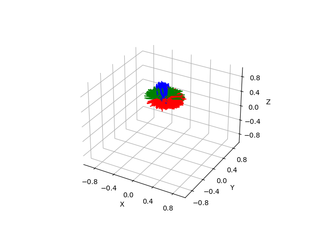
We can use estimate_gaussian_transform_from_samples() to estimate a Gaussian distribution of transformations. We can sample from a known Gaussian distribution of transformations with random_transform() as illustrated in the Example Sample Transforms.

9.2. Visualization of Uncertainty

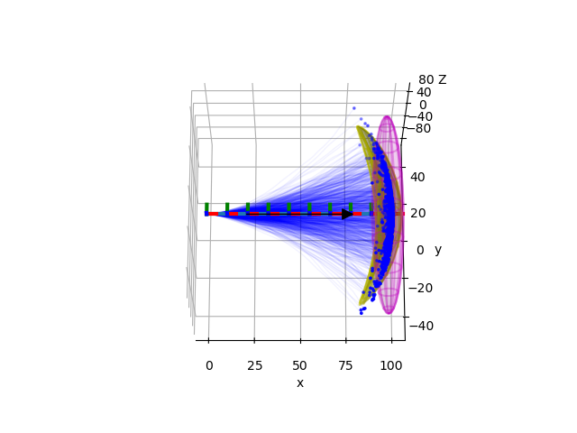
A typical visual representation of Gaussian distributions in 3D coordinates are equiprobable ellipsoids (obtained with to_ellipsoid()). This is equivalent to showing the \(k\sigma, k \in \mathbb{R}\) intervals of a 1D Gaussian distribution. However, for transformations there are also interactions between rotation and translation components so that an ellipsoid is not an appropriate representation to visualize the distribution of transformations in 3D. We have to project a 6D hyper-ellipsoid to 3D (for which we can use to_projected_ellipsoid()), which can result in banana-like shapes.

9.3. Concatenation of Uncertain Transformations

There are two different ways of defining uncertainty of transformations when we concatenate multiple transformations. We can define uncertainty in the global frame of reference or in the local frame of reference and it makes a difference.

Global frame of reference (concat_globally_uncertain_transforms()):

\[Exp(_C\boldsymbol{\xi'}) \overline{\boldsymbol{T}}_{CA} = Exp(_C\boldsymbol{\xi}) \overline{\boldsymbol{T}}_{CB} Exp(_B\boldsymbol{\xi}) \overline{\boldsymbol{T}}_{BA},\]

where \(_B\boldsymbol{\xi} \sim \mathcal{N}(\boldsymbol{0}, \boldsymbol{\Sigma}_{BA})\), \(_C\boldsymbol{\xi} \sim \mathcal{N}(\boldsymbol{0}, \boldsymbol{\Sigma}_{CB})\), and \(_C\boldsymbol{\xi'} \sim \mathcal{N}(\boldsymbol{0}, \boldsymbol{\Sigma}_{CA})\).

This method of concatenating uncertain transformation is used in Example Concatenate Uncertain Transforms, which illustrates how the banana distribution is generated.

Local frame of reference (concat_locally_uncertain_transforms()):

\[\overline{\boldsymbol{T}}_{CA} Exp(_A\boldsymbol{\xi'}) = \overline{\boldsymbol{T}}_{CB} Exp(_B\boldsymbol{\xi}) \overline{\boldsymbol{T}}_{BA} Exp(_A\boldsymbol{\xi}),\]

where \(_B\boldsymbol{\xi} \sim \mathcal{N}(\boldsymbol{0}, \boldsymbol{\Sigma}_B)\), \(_A\boldsymbol{\xi} \sim \mathcal{N}(\boldsymbol{0}, \boldsymbol{\Sigma}_A)\), and \(_A\boldsymbol{\xi'} \sim \mathcal{N}(\boldsymbol{0}, \boldsymbol{\Sigma}_{A,total})\).

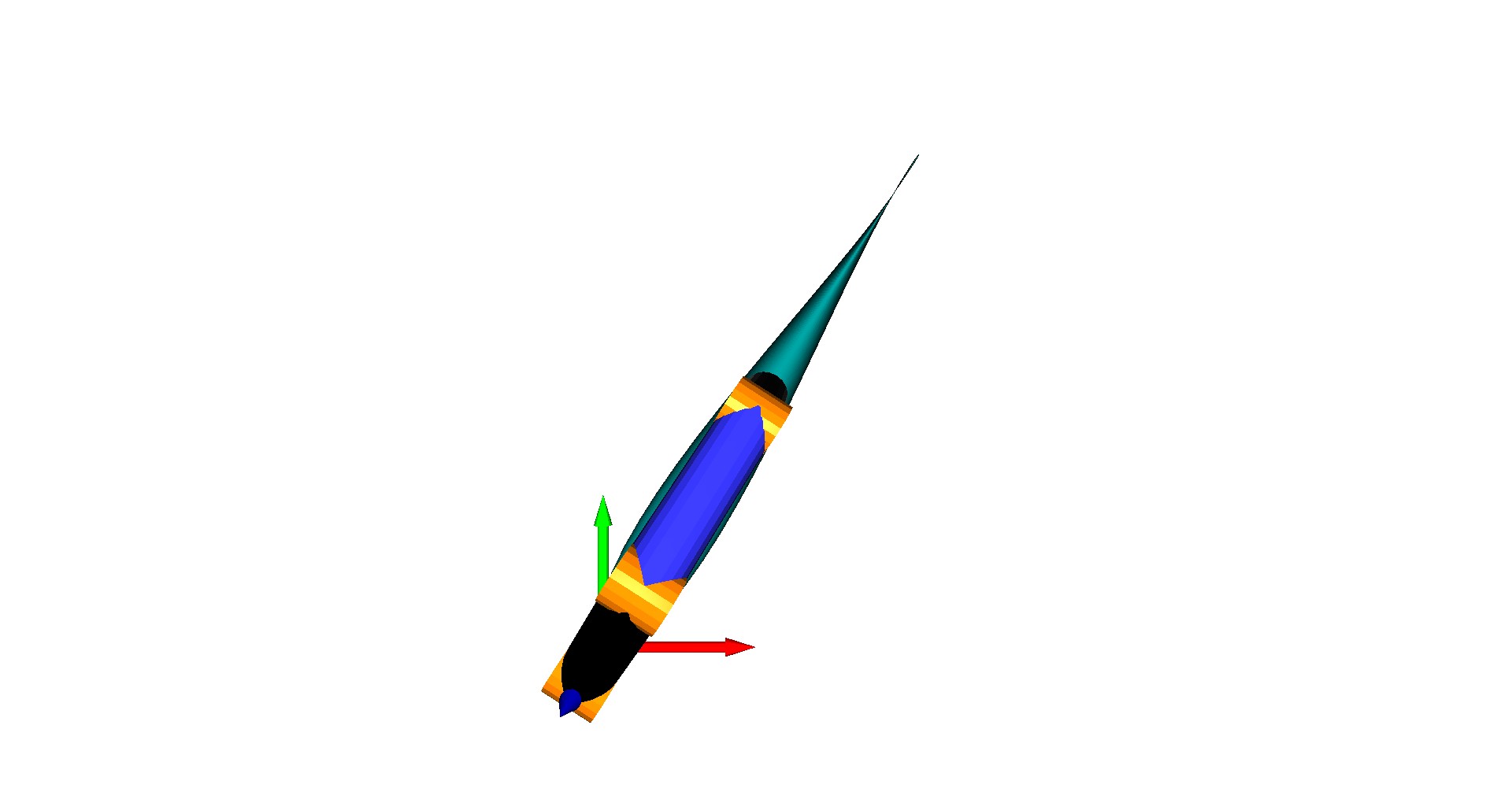
This method of concatenating uncertain transformations is used in Example Probabilistic Product of Exponentials, which illustrates probabilistic robot kinematics.

9.4. Fusion of Uncertain Poses

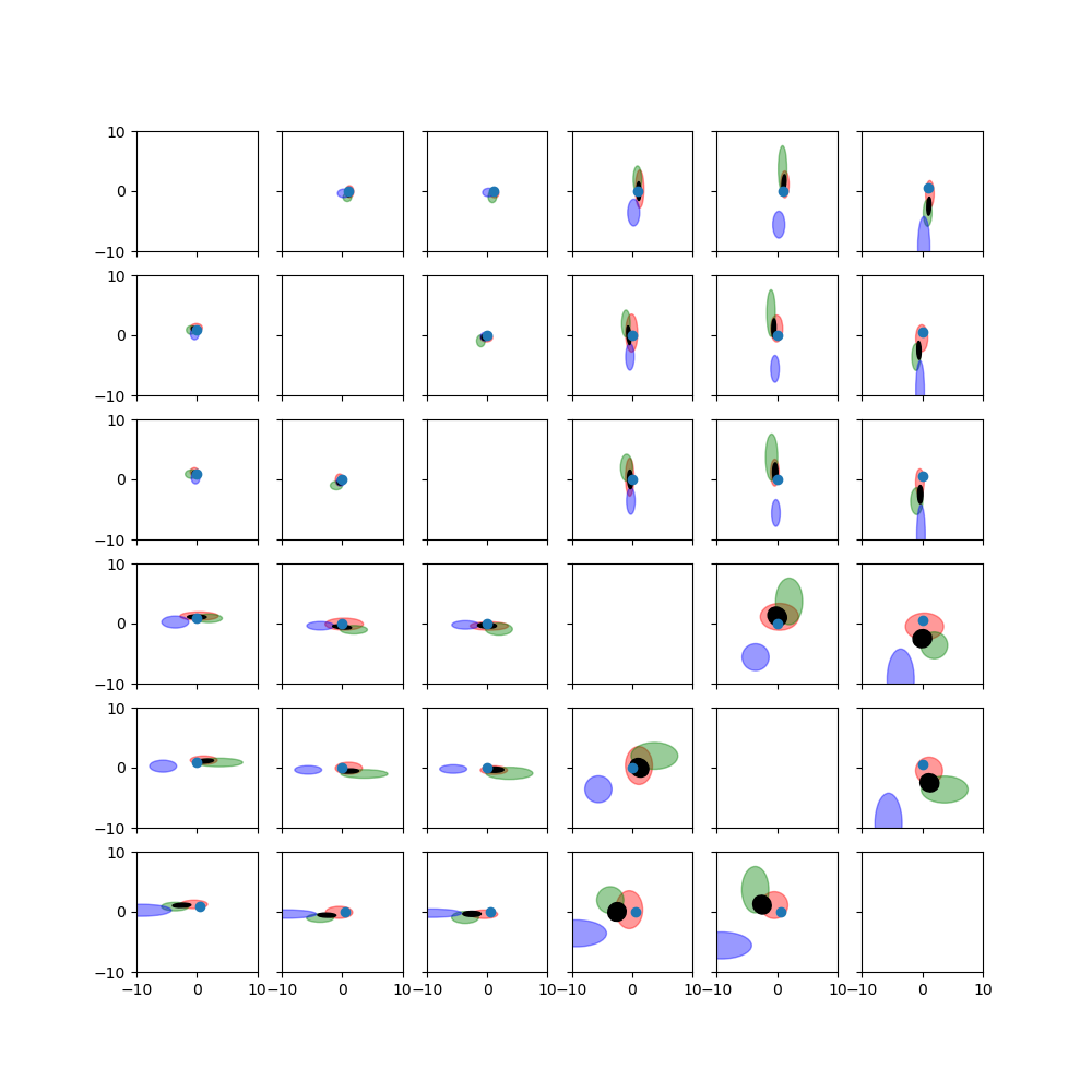
Fusing of multiple uncertain poses with pose_fusion() is required, for instance, in state estimation and sensor fusion. The Example Fuse 3 Poses illustrates this process.