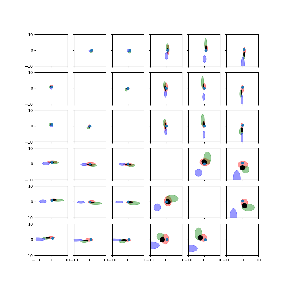
Fuse 3 Poses

Each of the poses has an associated covariance that is considered during the fusion. Each of the plots shows a projection of the distributions in exponential coordinate space to two dimensions. Red, green, and blue ellipses represent the uncertain poses that will be fused. A black ellipse indicates the fused pose’s distribution.

This example is from

Barfoot, Furgale: Associating Uncertainty With Three-Dimensional Poses for Use in Estimation Problems, http://ncfrn.mcgill.ca/members/pubs/barfoot_tro14.pdf

import matplotlib.pyplot as plt
import numpy as np

import pytransform3d.transformations as pt
import pytransform3d.uncertainty as pu

Helper Functions

Here you find some helper functions for plotting.

def to_ellipse(cov, factor=1.0):
    """Compute error ellipse.

    An error ellipse shows equiprobable points of a 2D Gaussian distribution.

    Parameters
    ----------
    cov : array-like, shape (2, 2)
        Covariance of the Gaussian distribution.

    factor : float, optional (default: 1)
        One means standard deviation.

    Returns
    -------
    angle : float
        Rotation angle of the ellipse.

    width : float
        Width of the ellipse (semi axis, not diameter).

    height : float
        Height of the ellipse (semi axis, not diameter).
    """
    from scipy import linalg

    vals, vecs = linalg.eigh(cov)
    order = vals.argsort()[::-1]
    vals, vecs = vals[order], vecs[:, order]
    angle = np.arctan2(*vecs[:, 0][::-1])
    width, height = factor * np.sqrt(vals)
    return angle, width, height


def plot_error_ellipse(
    ax, mean, cov, color=None, alpha=0.25, factors=np.linspace(0.25, 2.0, 8)
):
    """Plot error ellipse of MVN.

    Parameters
    ----------
    ax : axis
        Matplotlib axis.

    mean : array-like, shape (2,)
        Mean of the Gaussian distribution.

    cov : array-like, shape (2, 2)
        Covariance of the Gaussian distribution.

    color : str, optional (default: None)
        Color in which the ellipse should be plotted

    alpha : float, optional (default: 0.25)
        Alpha value for ellipse

    factors : array, optional (default: np.linspace(0.25, 2.0, 8))
        Multiples of the standard deviations that should be plotted.
    """
    from matplotlib.patches import Ellipse

    for factor in factors:
        angle, width, height = to_ellipse(cov, factor)
        ell = Ellipse(
            xy=mean,
            width=2.0 * width,
            height=2.0 * height,
            angle=np.degrees(angle),
        )
        ell.set_alpha(alpha)
        if color is not None:
            ell.set_color(color)
        ax.add_artist(ell)

Example Configuration

A ground truth pose is known in this example. We sample 3 poses with different covariances around the ground truth pose.

x_true = np.array([1.0, 0.0, 0.0, 0.0, 0.0, np.pi / 6.0])
T_true = pt.transform_from_exponential_coordinates(x_true)
alpha = 5.0
cov1 = alpha * np.diag([0.1, 0.2, 0.1, 2.0, 1.0, 1.0])
cov2 = alpha * np.diag([0.1, 0.1, 0.2, 1.0, 3.0, 1.0])
cov3 = alpha * np.diag([0.2, 0.1, 0.1, 1.0, 1.0, 5.0])

rng = np.random.default_rng(0)

T1 = np.dot(
    pt.transform_from_exponential_coordinates(
        pt.random_exponential_coordinates(rng=rng, cov=cov1)
    ),
    T_true,
)
T2 = np.dot(
    pt.transform_from_exponential_coordinates(
        pt.random_exponential_coordinates(rng=rng, cov=cov2)
    ),
    T_true,
)
T3 = np.dot(
    pt.transform_from_exponential_coordinates(
        pt.random_exponential_coordinates(rng=rng, cov=cov3)
    ),
    T_true,
)

x1 = pt.exponential_coordinates_from_transform(T1)
x2 = pt.exponential_coordinates_from_transform(T2)
x3 = pt.exponential_coordinates_from_transform(T3)

Fusion

We can then fuse the 3 sampled poses with their associated covariances.

T_est, cov_est, V = pu.pose_fusion([T1, T2, T3], [cov1, cov2, cov3])

Plotting

Each subplot shows two dimensions of the exponential coordinate space. Each sampled pose and its associated covariance matrix is displayed as an equiprobable ellipse. The fused pose estimate is also shown with its associated covariance as an equiprobable ellipse. For comparison, the ground truth pose is shown as a point.

x_est = pt.exponential_coordinates_from_transform(T_est)
_, axes = plt.subplots(
    nrows=6, ncols=6, sharex=True, sharey=True, squeeze=True, figsize=(10, 10)
)
factors = [1.0]
for i in range(6):
    for j in range(6):
        if i == j:
            continue

        indices = np.array([i, j])
        ax = axes[i][j]

        for x, cov, color in zip([x1, x2, x3], [cov1, cov2, cov3], "rgb"):
            plot_error_ellipse(
                ax,
                x[indices],
                cov[indices][:, indices],
                color=color,
                alpha=0.4,
                factors=factors,
            )

        plot_error_ellipse(
            ax,
            x_est[indices],
            cov_est[indices][:, indices],
            color="k",
            alpha=1,
            factors=factors,
        )

        ax.scatter(x_true[i], x_true[j])

        ax.set_xlim((-10, 10))
        ax.set_ylim((-10, 10))

plt.show()