Concatenate Uncertain Transforms

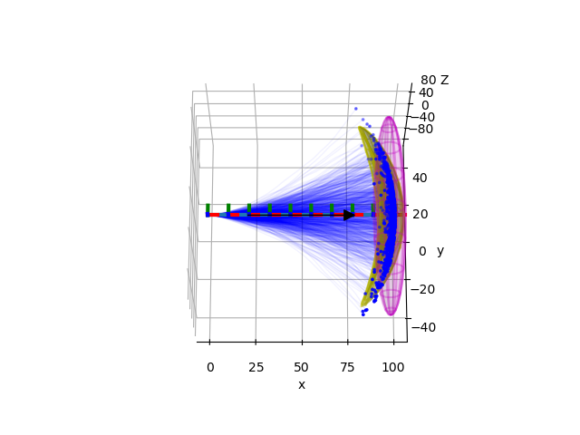
Each of the poses has an associated covariance that is considered. In this example, we assume that a robot is moving with constant velocity along the x-axis, however, there is noise in the orientation of the robot that accumulates and leads to different paths when sampling. Uncertainty accumulation leads to the so-called banana distribution, which does not seem Gaussian in Cartesian space, but it is Gaussian in exponential coordinate space of SO(3).

This example adapted and modified to 3D from

Barfoot, Furgale: Associating Uncertainty With Three-Dimensional Poses for Use in Estimation Problems, http://ncfrn.mcgill.ca/members/pubs/barfoot_tro14.pdf

The banana distribution was analyzed in detail by

Long, Wolfe, Mashner, Chirikjian: The Banana Distribution is Gaussian: A Localization Study with Exponential Coordinates, http://www.roboticsproceedings.org/rss08/p34.pdf

import numpy as np
import matplotlib.pyplot as plt
import pytransform3d.transformations as pt
import pytransform3d.trajectories as ptr
import pytransform3d.uncertainty as pu
import pytransform3d.plot_utils as ppu


rng = np.random.default_rng(0)
cov_pose_chol = np.diag([0, 0.02, 0.03, 0, 0, 0])
cov_pose = np.dot(cov_pose_chol, cov_pose_chol.T)
velocity_vector = np.array([0, 0, 0, 1.0, 0, 0])
T_vel = pt.transform_from_exponential_coordinates(velocity_vector)
n_steps = 100
n_mc_samples = 1000
n_skip_trajectories = 1  # plot every n-th trajectory

T_est = np.eye(4)
path = np.zeros((n_steps + 1, 6))
path[0] = pt.exponential_coordinates_from_transform(T_est)
cov_est = np.zeros((6, 6))
for t in range(n_steps):
    T_est, cov_est = pu.concat_globally_uncertain_transforms(
        T_est, cov_est, T_vel, cov_pose)
    path[t + 1] = pt.exponential_coordinates_from_transform(T_est)

T = np.eye(4)
mc_path = np.zeros((n_steps + 1, n_mc_samples, 4, 4))
mc_path[0, :] = T
for t in range(n_steps):
    noise_samples = ptr.transforms_from_exponential_coordinates(
        cov_pose_chol.dot(rng.standard_normal(size=(6, n_mc_samples))).T)
    step_samples = ptr.concat_many_to_one(noise_samples, T_vel)
    mc_path[t + 1] = np.einsum("nij,njk->nik", step_samples, mc_path[t])
# Plot the random samples' trajectory lines (in a frame attached to the start)
# same as mc_path[t, i, :3, :3].T.dot(mc_path[t, i, :3, 3]), but faster
mc_path_vec = np.einsum(
    "tinm,tin->tim", mc_path[:, :, :3, :3], mc_path[:, :, :3, 3])

ax = ppu.make_3d_axis(100)

for i in range(0, mc_path_vec.shape[1], n_skip_trajectories):
    ax.plot(
        mc_path_vec[:, i, 0], mc_path_vec[:, i, 1], mc_path_vec[:, i, 2],
        lw=1, c="b", alpha=0.05)
ax.scatter(
    mc_path_vec[-1, :, 0], mc_path_vec[-1, :, 1], mc_path_vec[-1, :, 2],
    s=3, c="b")

ptr.plot_trajectory(ax, ptr.pqs_from_transforms(
    ptr.transforms_from_exponential_coordinates(path)), s=5.0, lw=3)

pu.plot_projected_ellipsoid(
    ax, T_est, cov_est, wireframe=False, alpha=0.3, color="y", factor=3.0)
pu.plot_projected_ellipsoid(
    ax, T_est, cov_est, wireframe=True, alpha=0.5, color="y", factor=3.0)

mean_mc = np.mean(mc_path_vec[-1, :], axis=0)
cov_mc = np.cov(mc_path_vec[-1, :], rowvar=False)

ellipsoid2origin, radii = pu.to_ellipsoid(mean_mc, cov_mc)
ppu.plot_ellipsoid(
    ax, 3.0 * radii, ellipsoid2origin, wireframe=False, alpha=0.1, color="m")
ppu.plot_ellipsoid(
    ax, 3.0 * radii, ellipsoid2origin, wireframe=True, alpha=0.3, color="m")

plt.xlim((-5, 105))
plt.ylim((-50, 50))
plt.xlabel("x")
plt.ylabel("y")
ax.view_init(elev=70, azim=-90)
plt.show()