Invert Uncertain Transform

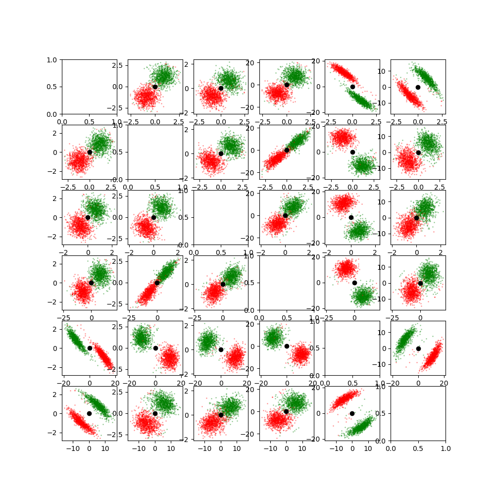
We sample from the original transform distribution and from the inverse distribution. Samples are then projected to all 2D planes and plotted. The color indicates the pose distribution. Green is the original distribution and red is the inverse.

import numpy as np
import matplotlib.pyplot as plt
import pytransform3d.uncertainty as pu
import pytransform3d.rotations as pr
import pytransform3d.transformations as pt
import pytransform3d.trajectories as ptr


n_mc_samples = 1000
rng = np.random.default_rng(1)
alpha = 2.0

A2B = pt.transform_from(
    R=pr.matrix_from_euler([1.5, 0.5, 1.3], 0, 1, 2, True),
    p=[10.0, -7.0, -5.0]
)
variances = alpha * np.array([0.1, 0.2, 0.1, 2.0, 1.0, 1.0])
std_devs = np.sqrt(variances)
correlations = np.array([
    [0.5, 0, 0, 0, 0, 0],
    [0.1, 0.5, 0, 0, 0, 0],
    [-0.3, 0.1, 0.5, 0, 0, 0],
    [-0.1, 0.2, 0.3, 0.5, 0, 0],
    [-0.3, -0.1, -0.2, 0.3, 0.5, 0],
    [-0.1, 0.1, 0.2, 0.1, 0.3, 0.5]
])
correlations += correlations.T
cov_A2B = correlations * np.outer(std_devs, std_devs)
x_A2B = pt.exponential_coordinates_from_transform(A2B)
samples_A2B = ptr.exponential_coordinates_from_transforms(
    [pt.random_transform(rng, A2B, cov_A2B) for _ in range(n_mc_samples)])

B2A, cov_B2A = pu.invert_uncertain_transform(A2B, cov_A2B)
x_B2A = pt.exponential_coordinates_from_transform(B2A)
samples_B2A = ptr.exponential_coordinates_from_transforms(
    [pt.random_transform(rng, B2A, cov_B2A) for _ in range(n_mc_samples)])

_, axes = plt.subplots(nrows=6, ncols=6, squeeze=True, figsize=(10, 10))
for i in range(6):
    for j in range(6):
        if i == j:
            continue

        indices = np.array([i, j])
        ax = axes[i][j]

        ax.scatter(
            samples_A2B[:, i], samples_A2B[:, j], color="g", s=1, alpha=0.3)
        ax.scatter(
            samples_B2A[:, i], samples_B2A[:, j], color="r", s=1, alpha=0.3)

        ax.scatter(0, 0, color="k")

plt.show()