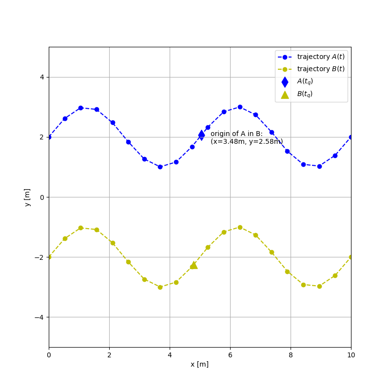
Managing Transformations over Time

In this example, given two trajectories of 3D rigid transformations, we will interpolate both and use the transform manager for the target timestep.

/home/afabisch/Data/Projects/pytransform3d/pytransform3d/examples/plots/plot_interpolation_for_transform_manager.py:39: DeprecationWarning: function is deprecated, use matrix_from_euler
  R = pr.active_matrix_from_extrinsic_euler_zyx([yaw[i], 0, 0])

import matplotlib.pyplot as plt
import numpy as np

from pytransform3d import rotations as pr
from pytransform3d import transformations as pt
from pytransform3d.transform_manager import (
    TemporalTransformManager,
    NumpyTimeseriesTransform,
)


def create_sinusoidal_movement(
    duration_sec, sample_period, x_velocity, y_start_offset, start_time
):
    """Create a planar (z=0) sinusoidal movement around x-axis."""
    time = np.arange(0, duration_sec, sample_period) + start_time
    n_steps = len(time)
    x = np.linspace(0, x_velocity * duration_sec, n_steps)

    spatial_freq = 1.0 / 5.0  # 1 sinus per 5m
    omega = 2.0 * np.pi * spatial_freq
    y = np.sin(omega * x)
    y += y_start_offset

    dydx = omega * np.cos(omega * x)
    yaw = np.arctan2(dydx, np.ones_like(dydx))

    pqs = []
    for i in range(n_steps):
        R = pr.active_matrix_from_extrinsic_euler_zyx([yaw[i], 0, 0])
        T = pt.transform_from(R, [x[i], y[i], 0])
        pq = pt.pq_from_transform(T)
        pqs.append(pq)

    return time, np.array(pqs)


# create entities A and B together with their transformations from world
duration = 10.0  # [s]
sample_period = 0.5  # [s]
velocity_x = 1  # [m/s]
time_A, pqs_A = create_sinusoidal_movement(
    duration, sample_period, velocity_x, y_start_offset=2.0, start_time=0.1
)
time_B, pqs_B = create_sinusoidal_movement(
    duration, sample_period, velocity_x, y_start_offset=-2.0, start_time=0.35
)

# package them into an instance of `TimeVaryingTransform` abstract class
transform_WA = NumpyTimeseriesTransform(time_A, pqs_A)
transform_WB = NumpyTimeseriesTransform(time_B, pqs_B)

tm = TemporalTransformManager()

tm.add_transform("A", "world", transform_WA)
tm.add_transform("B", "world", transform_WB)

query_time = 4.9  # [s] or an array of times np.array([4.9, 5.2])
A2B_at_query_time = tm.get_transform_at_time("A", "B", query_time)

# transform the origin of A in A (x=0, y=0, z=0) to B
origin_of_A_pos = pt.vector_to_point([0, 0, 0])
origin_of_A_in_B_xyz = pt.transform(A2B_at_query_time, origin_of_A_pos)[:-1]

# for visualization purposes
pq_A = pt.pq_from_transform(transform_WA.as_matrix(query_time))
pq_B = pt.pq_from_transform(transform_WB.as_matrix(query_time))

plt.figure(figsize=(8, 8))
plt.plot(pqs_A[:, 0], pqs_A[:, 1], "bo--", label="trajectory $A(t)$")
plt.plot(pqs_B[:, 0], pqs_B[:, 1], "yo--", label="trajectory $B(t)$")
plt.scatter(pq_A[0], pq_A[1], color="b", s=120, marker="d", label="$A(t_q)$")
plt.scatter(pq_B[0], pq_B[1], color="y", s=120, marker="^", label="$B(t_q)$")
plt.text(
    pq_A[0] + 0.3,
    pq_A[1] - 0.3,
    f"origin of A in B:\n(x={origin_of_A_in_B_xyz[0]:.2f}m,"
    + f" y={origin_of_A_in_B_xyz[1]:.2f}m)",
)
plt.xlabel("x [m]")
plt.ylabel("y [m]")
plt.xlim(0, 10)
plt.ylim(-5, 5)
plt.grid()
plt.legend()
plt.show()