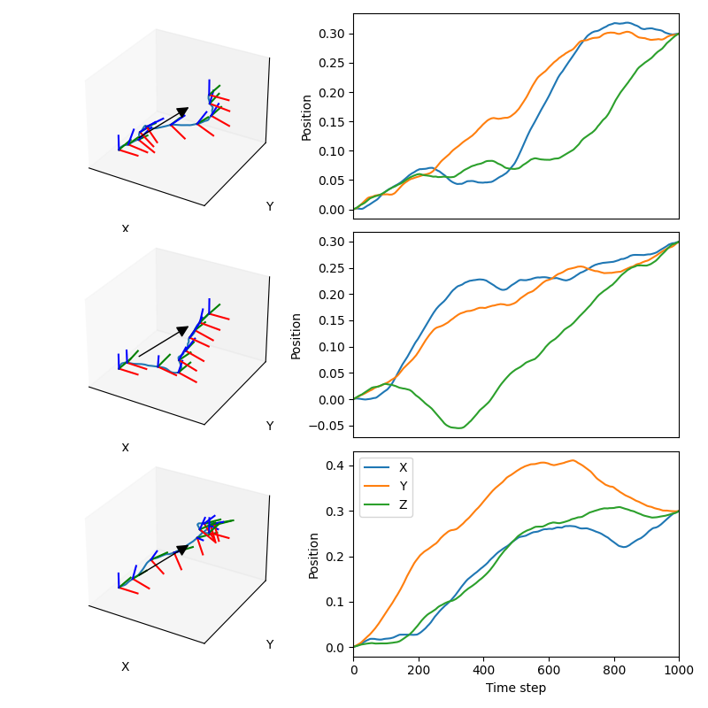
Random Trajectories

These plots show several randomly generated trajectories. Each row shows a different trajectory. On the left side you can see the position and orientation represented by small coordinate frames. On the right side you can see the positions over time.

import matplotlib.pyplot as plt
import numpy as np

import pytransform3d.trajectories as ptr
import pytransform3d.transformations as pt

We sample three random trajectories.

n_trajectories = 3
trajectories = ptr.random_trajectories(
    rng=np.random.default_rng(5),
    n_trajectories=n_trajectories,
    n_steps=1001,
    start=np.eye(4),
    goal=pt.transform_from(R=np.eye(3), p=0.3 * np.ones(3)),
    scale=[200] * 3 + [50] * 3,
)

We plot the trajectory in 3D on the left and in 2D on the right.

plt.figure(figsize=(8, 8))
for i in range(n_trajectories):
    ax = plt.subplot(n_trajectories, 2, 1 + 2 * i, projection="3d")
    plt.setp(
        ax,
        xlim=(-0.1, 0.5),
        ylim=(-0.1, 0.5),
        zlim=(-0.1, 0.5),
        xlabel="X",
        ylabel="Y",
    )
    ax.set_xticks(())
    ax.set_yticks(())
    ax.set_zticks(())
    ptr.plot_trajectory(
        ax=ax, P=ptr.pqs_from_transforms(trajectories[i]), s=0.1
    )

    ax = plt.subplot(n_trajectories, 2, 2 + 2 * i)
    for d in range(3):
        plt.plot(trajectories[i, :, d, 3].T, label="XYZ"[d])
    if i != n_trajectories - 1:
        ax.set_xticks(())
    else:
        ax.set_xlabel("Time step")
        ax.legend(loc="best")
    ax.set_ylabel("Position")
    ax.set_xlim((0, trajectories.shape[1] - 1))

plt.tight_layout()
plt.show()