pytransform3d.visualizer.Figure¶

class pytransform3d.visualizer.Figure(window_name='Open3D', width=1920, height=1080, with_key_callbacks=False)[source]¶

Bases: object

The top level container for all the plot elements.

You can close the visualizer with the keys escape or q.

Parameters:

window_namestr, optional (default: Open3D): Window title name.
widthint, optional (default: 1920): Width of the window.
heightint, optional (default: 1080): Height of the window.
with_key_callbacksbool, optional (default: False): Creates a visualizer that allows to register callbacks for keys.

__init__(window_name='Open3D', width=1920, height=1080, with_key_callbacks=False)[source]¶

Methods

`__init__`([window_name, width, height, ...])
`add_geometry`(geometry)	Add geometry to visualizer.
`animate`(callback, n_frames[, loop, fargs])	Make animation with callback.
`plot`(P[, c])	Plot line.
`plot_basis`([R, p, s, strict_check])	Plot basis.
`plot_box`([size, A2B, c])	Plot box.
`plot_camera`(M[, cam2world, ...])	Plot camera in world coordinates.
`plot_capsule`([height, radius, A2B, ...])	Plot capsule.
`plot_cone`([height, radius, A2B, resolution, c])	Plot cone.
`plot_cylinder`([length, radius, A2B, ...])	Plot cylinder.
`plot_ellipsoid`([radii, A2B, resolution, c])	Plot ellipsoid.
`plot_graph`(tm, frame[, show_frames, ...])	Plot graph of connected frames.
`plot_mesh`(filename[, A2B, s, c])	Plot mesh.
`plot_plane`([normal, d, point_in_plane, s, c])	Plot plane.
`plot_sphere`([radius, A2B, resolution, c])	Plot sphere.
`plot_trajectory`(P[, n_frames, s, c])	Trajectory of poses.
`plot_transform`([A2B, s, name, strict_check])	Plot coordinate frame.
`plot_vector`([start, direction, c])	Plot vector.
`remove_artist`(artist)	Remove artist from visualizer.
`save_image`(filename)	Save rendered image to file.
`scatter`(P[, s, c])	Plot collection of points.
`set_line_width`(line_width)	Set render option line width.
`set_zoom`(zoom)	Set zoom.
`show`()	Display the figure window.
`update_geometry`(geometry)	Indicate that geometry has been updated.
`view_init`([azim, elev])	Set the elevation and azimuth of the axes.

add_geometry(geometry)[source]¶

Add geometry to visualizer.

Parameters:

geometryGeometry: Open3D geometry.

update_geometry(geometry)[source]¶

Indicate that geometry has been updated.

Parameters:

geometryGeometry: Open3D geometry.

remove_artist(artist)[source]¶

Remove artist from visualizer.

Parameters:

artistArtist: Artist that should be removed from this figure.

set_line_width(line_width)[source]¶

Set render option line width.

Note: this feature does not work in Open3D’s visualizer at the moment.

Parameters:

line_widthfloat: Line width.

set_zoom(zoom)[source]¶

Set zoom.

Parameters:

zoomfloat: Zoom of the visualizer.

animate(callback, n_frames, loop=False, fargs=())[source]¶

Make animation with callback.

Parameters:

callbackcallable: Callback that will be called in a loop to update geometries. The first input of the function will be the current frame index from [0, n_frames). Further arguments can be given as fargs. The function should return one artist object or a list of artists that have been updated.
n_framesint: Total number of frames.
loopbool, optional (default: False): Run callback in an infinite loop.
fargslist, optional (default: []): Arguments that will be passed to the callback.

Raises:

RuntimeError: When callback does not return any artists

view_init(azim=- 60, elev=30)[source]¶

Set the elevation and azimuth of the axes.

Parameters:

azimfloat, optional (default: -60): Azimuth angle in the x,y plane in degrees.
elevfloat, optional (default: 30): Elevation angle in the z plane.

plot(P, c=(0, 0, 0))[source]¶

Plot line.

Parameters:

Parray-like, shape (n_points, 3): Points of which the line consists.
carray-like, shape (n_points - 1, 3) or (3,), optional (default: black): Color can be given as individual colors per line segment or as one color for each segment. A color is represented by 3 values between 0 and 1 indicate representing red, green, and blue respectively.

Returns:

lineLine3D: New line.

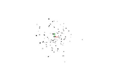
scatter(P, s=0.05, c=None)[source]¶

Plot collection of points.

Parameters:

Parray, shape (n_points, 3): Points
sfloat, optional (default: 0.05): Scaling of the spheres that will be drawn.
carray-like, shape (3,) or (n_points, 3), optional (default: black): A color is represented by 3 values between 0 and 1 indicate representing red, green, and blue respectively.

Returns:

point_collectionPointCollection3D: New point collection.

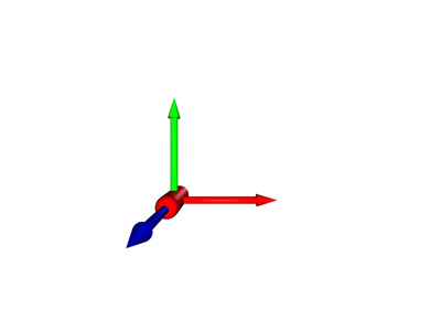
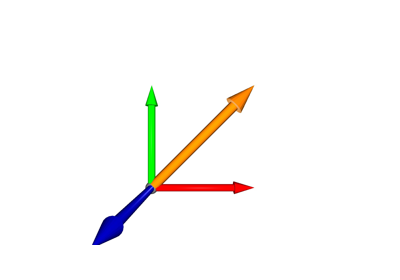
plot_vector(start=array([0., 0., 0.]), direction=array([1, 0, 0]), c=(0, 0, 0))[source]¶

Plot vector.

Parameters:

startarray-like, shape (3,), optional (default: [0, 0, 0]): Start of the vector
directionarray-like, shape (3,), optional (default: [1, 0, 0]): Direction of the vector
carray-like, shape (3,), optional (default: black): A color is represented by 3 values between 0 and 1 indicate representing red, green, and blue respectively.

Returns:

vectorVector3D: New vector.

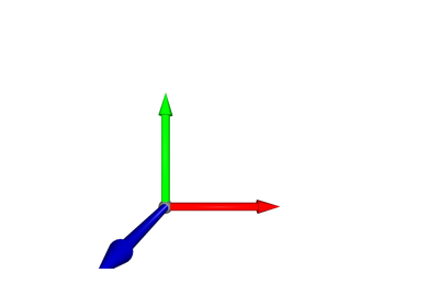
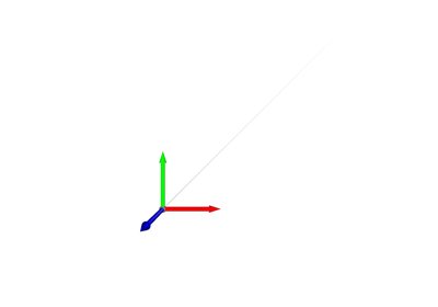
plot_basis(R=None, p=array([0., 0., 0.]), s=1.0, strict_check=True)[source]¶

Plot basis.

Parameters:

Rarray-like, shape (3, 3), optional (default: I): Rotation matrix, each column contains a basis vector
parray-like, shape (3,), optional (default: [0, 0, 0]): Offset from the origin
sfloat, optional (default: 1): Scaling of the frame that will be drawn
strict_checkbool, optional (default: True): Raise a ValueError if the rotation matrix is not numerically close enough to a real rotation matrix. Otherwise we print a warning.

Returns:

Frameframe: New frame.

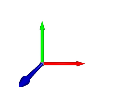
plot_transform(A2B=None, s=1.0, name=None, strict_check=True)[source]¶

Plot coordinate frame.

Parameters:

A2Barray-like, shape (4, 4): Transform from frame A to frame B
sfloat, optional (default: 1): Length of basis vectors
namestr, optional (default: None): Name of the frame
strict_checkbool, optional (default: True): Raise a ValueError if the transformation matrix is not numerically close enough to a real transformation matrix. Otherwise we print a warning.

Returns:

Frameframe: New frame.

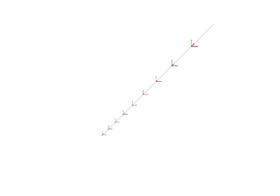
plot_trajectory(P, n_frames=10, s=1.0, c=(0, 0, 0))[source]¶

Trajectory of poses.

Parameters:

Parray-like, shape (n_steps, 7), optional (default: None): Sequence of poses represented by positions and quaternions in the order (x, y, z, w, vx, vy, vz) for each step
n_framesint, optional (default: 10): Number of frames that should be plotted to indicate the rotation
sfloat, optional (default: 1): Scaling of the frames that will be drawn
carray-like, shape (3,), optional (default: black): A color is represented by 3 values between 0 and 1 indicate representing red, green, and blue respectively.

Returns:

trajectoryTrajectory: New trajectory.

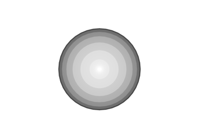
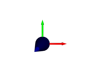
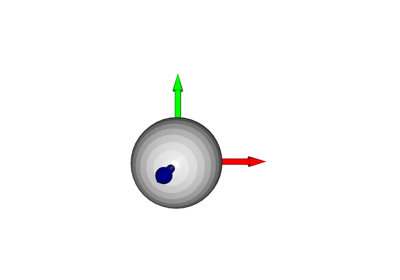
plot_sphere(radius=1.0, A2B=array([[1., 0., 0., 0.], [0., 1., 0., 0.], [0., 0., 1., 0.], [0., 0., 0., 1.]]), resolution=20, c=None)[source]¶

Plot sphere.

Parameters:

radiusfloat, optional (default: 1): Radius of the sphere
A2Barray-like, shape (4, 4): Transform from frame A to frame B
resolutionint, optional (default: 20): The resolution of the sphere. The longitudes will be split into resolution segments (i.e. there are resolution + 1 latitude lines including the north and south pole). The latitudes will be split into 2 * resolution segments (i.e. there are 2 * resolution longitude lines.)
carray-like, shape (3,), optional (default: None): Color

Returns:

sphereSphere: New sphere.

plot_box(size=array([1., 1., 1.]), A2B=array([[1., 0., 0., 0.], [0., 1., 0., 0.], [0., 0., 1., 0.], [0., 0., 0., 1.]]), c=None)[source]¶

Plot box.

Parameters:

sizearray-like, shape (3,), optional (default: [1, 1, 1]): Size of the box per dimension
A2Barray-like, shape (4, 4), optional (default: I): Center of the box
carray-like, shape (3,), optional (default: None): Color

Returns:

boxBox: New box.

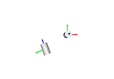
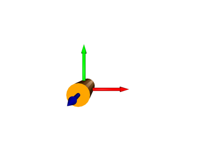
plot_cylinder(length=2.0, radius=1.0, A2B=array([[1., 0., 0., 0.], [0., 1., 0., 0.], [0., 0., 1., 0.], [0., 0., 0., 1.]]), resolution=20, split=4, c=None)[source]¶

Plot cylinder.

Parameters:

lengthfloat, optional (default: 1): Length of the cylinder.
radiusfloat, optional (default: 1): Radius of the cylinder.
A2Barray-like, shape (4, 4): Pose of the cylinder. The position corresponds to the center of the line segment and the z-axis to the direction of the line segment.
resolutionint, optional (default: 20): The circle will be split into resolution segments
splitint, optional (default: 4): The height will be split into split segments
carray-like, shape (3,), optional (default: None): Color

Returns:

cylinderCylinder: New cylinder.

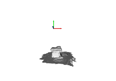
plot_mesh(filename, A2B=array([[1., 0., 0., 0.], [0., 1., 0., 0.], [0., 0., 1., 0.], [0., 0., 0., 1.]]), s=array([1., 1., 1.]), c=None)[source]¶

Plot mesh.

Parameters:

filenamestr: Path to mesh file
A2Barray-like, shape (4, 4): Center of the mesh
sarray-like, shape (3,), optional (default: [1, 1, 1]): Scaling of the mesh that will be drawn
carray-like, shape (n_vertices, 3) or (3,), optional (default: None): Color(s)

Returns:

meshMesh: New mesh.

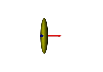
plot_ellipsoid(radii=array([1., 1., 1.]), A2B=array([[1., 0., 0., 0.], [0., 1., 0., 0.], [0., 0., 1., 0.], [0., 0., 0., 1.]]), resolution=20, c=None)[source]¶

Plot ellipsoid.

Parameters:

radiiarray-like, shape (3,): Radii along the x-axis, y-axis, and z-axis of the ellipsoid.
A2Barray-like, shape (4, 4): Transform from frame A to frame B
resolutionint, optional (default: 20): The resolution of the ellipsoid. The longitudes will be split into resolution segments (i.e. there are resolution + 1 latitude lines including the north and south pole). The latitudes will be split into 2 * resolution segments (i.e. there are 2 * resolution longitude lines.)
carray-like, shape (3,), optional (default: None): Color

Returns:

ellipsoidEllipsoid: New ellipsoid.

plot_capsule(height=1, radius=1, A2B=array([[1., 0., 0., 0.], [0., 1., 0., 0.], [0., 0., 1., 0.], [0., 0., 0., 1.]]), resolution=20, c=None)[source]¶

Plot capsule.

A capsule is the volume covered by a sphere moving along a line segment.

Parameters:

heightfloat, optional (default: 1): Height of the capsule along its z-axis.
radiusfloat, optional (default: 1): Radius of the capsule.
A2Barray-like, shape (4, 4): Pose of the capsule. The position corresponds to the center of the line segment and the z-axis to the direction of the line segment.
resolutionint, optional (default: 20): The resolution of the capsule. The longitudes will be split into resolution segments (i.e. there are resolution + 1 latitude lines including the north and south pole). The latitudes will be split into 2 * resolution segments (i.e. there are 2 * resolution longitude lines.)
carray-like, shape (3,), optional (default: None): Color

Returns:

capsuleCapsule: New capsule.

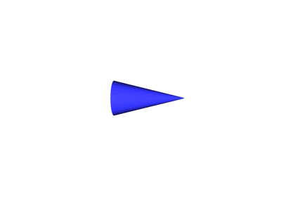
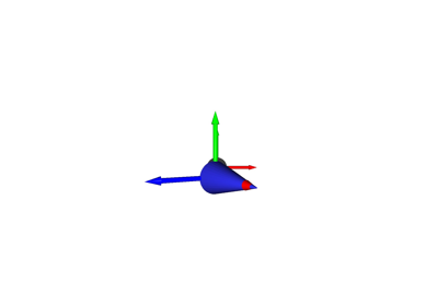
plot_cone(height=1, radius=1, A2B=array([[1., 0., 0., 0.], [0., 1., 0., 0.], [0., 0., 1., 0.], [0., 0., 0., 1.]]), resolution=20, c=None)[source]¶

Plot cone.

Parameters:

heightfloat, optional (default: 1): Height of the cone along its z-axis.
radiusfloat, optional (default: 1): Radius of the cone.
A2Barray-like, shape (4, 4): Pose of the cone.
resolutionint, optional (default: 20): The circle will be split into resolution segments.
carray-like, shape (3,), optional (default: None): Color

Returns:

coneCone: New cone.

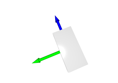
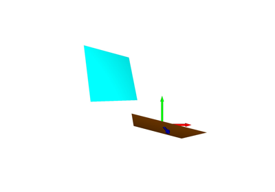
plot_plane(normal=array([0., 0., 1.]), d=None, point_in_plane=None, s=1.0, c=None)[source]¶

Plot plane.

Parameters:

normalarray-like, shape (3,), optional (default: [0, 0, 1]): Plane normal.
dfloat, optional (default: None): Distance to origin in Hesse normal form.
point_in_planearray-like, shape (3,), optional (default: None): Point in plane.
sfloat, optional (default: 1): Scaling of the plane that will be drawn.
carray-like, shape (3,), optional (default: None): Color.

Returns:

planePlane: New plane.

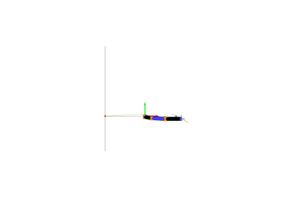
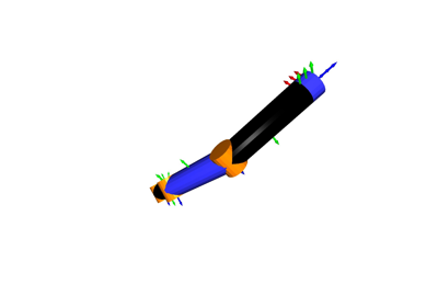
plot_graph(tm, frame, show_frames=False, show_connections=False, show_visuals=False, show_collision_objects=False, show_name=False, whitelist=None, convex_hull_of_collision_objects=False, s=1.0)[source]¶

Plot graph of connected frames.

Parameters:

tmTransformManager: Representation of the graph
framestr: Name of the base frame in which the graph will be displayed
show_framesbool, optional (default: False): Show coordinate frames
show_connectionsbool, optional (default: False): Draw lines between frames of the graph
show_visualsbool, optional (default: False): Show visuals that are stored in the graph
show_collision_objectsbool, optional (default: False): Show collision objects that are stored in the graph
show_namebool, optional (default: False): Show names of frames
whitelistlist, optional (default: all): List of frames that should be displayed
convex_hull_of_collision_objectsbool, optional (default: False): Show convex hull of collision objects.
sfloat, optional (default: 1): Scaling of the frames that will be drawn

Returns:

graphGraph: New graph.

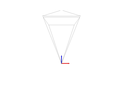
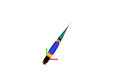
plot_camera(M, cam2world=None, virtual_image_distance=1, sensor_size=(1920, 1080), strict_check=True)[source]¶

Plot camera in world coordinates.

This function is inspired by Blender’s camera visualization. It will show the camera center, a virtual image plane, and the top of the virtual image plane.

Parameters:

Marray-like, shape (3, 3): Intrinsic camera matrix that contains the focal lengths on the diagonal and the center of the the image in the last column. It does not matter whether values are given in meters or pixels as long as the unit is the same as for the sensor size.
cam2worldarray-like, shape (4, 4), optional (default: I): Transformation matrix of camera in world frame. We assume that the position is given in meters.
virtual_image_distancefloat, optional (default: 1): Distance from pinhole to virtual image plane that will be displayed. We assume that this distance is given in meters. The unit has to be consistent with the unit of the position in cam2world.
sensor_sizearray-like, shape (2,), optional (default: [1920, 1080]): Size of the image sensor: (width, height). It does not matter whether values are given in meters or pixels as long as the unit is the same as for the sensor size.
strict_checkbool, optional (default: True): Raise a ValueError if the transformation matrix is not numerically close enough to a real transformation matrix. Otherwise we print a warning.

Returns: